MOC - Introduction to Statistics and Statistical Programming

Scale of measure

A finite data sequence $x_1,...,x_n$ with real data $x_i$ has values (unique values, sometimes called Item Expression) ${\xi }_1<...<{\xi }_k$ where $k\le n$ because the same value can be measured multiple times.

We interpret Stochastic Independence as causal independence, which means that we will look at the progression of data sequences to determine if they are independent of another.

Use Dichotomisation to make data usable for Runs test for long 01-sequence which determines whether a data sequence is random or not.

We want to be able to infer the underlying random mechanism of a data sequence. Ordered Data Sequences makes it a bit easier as the order usually doesn’t play a role.

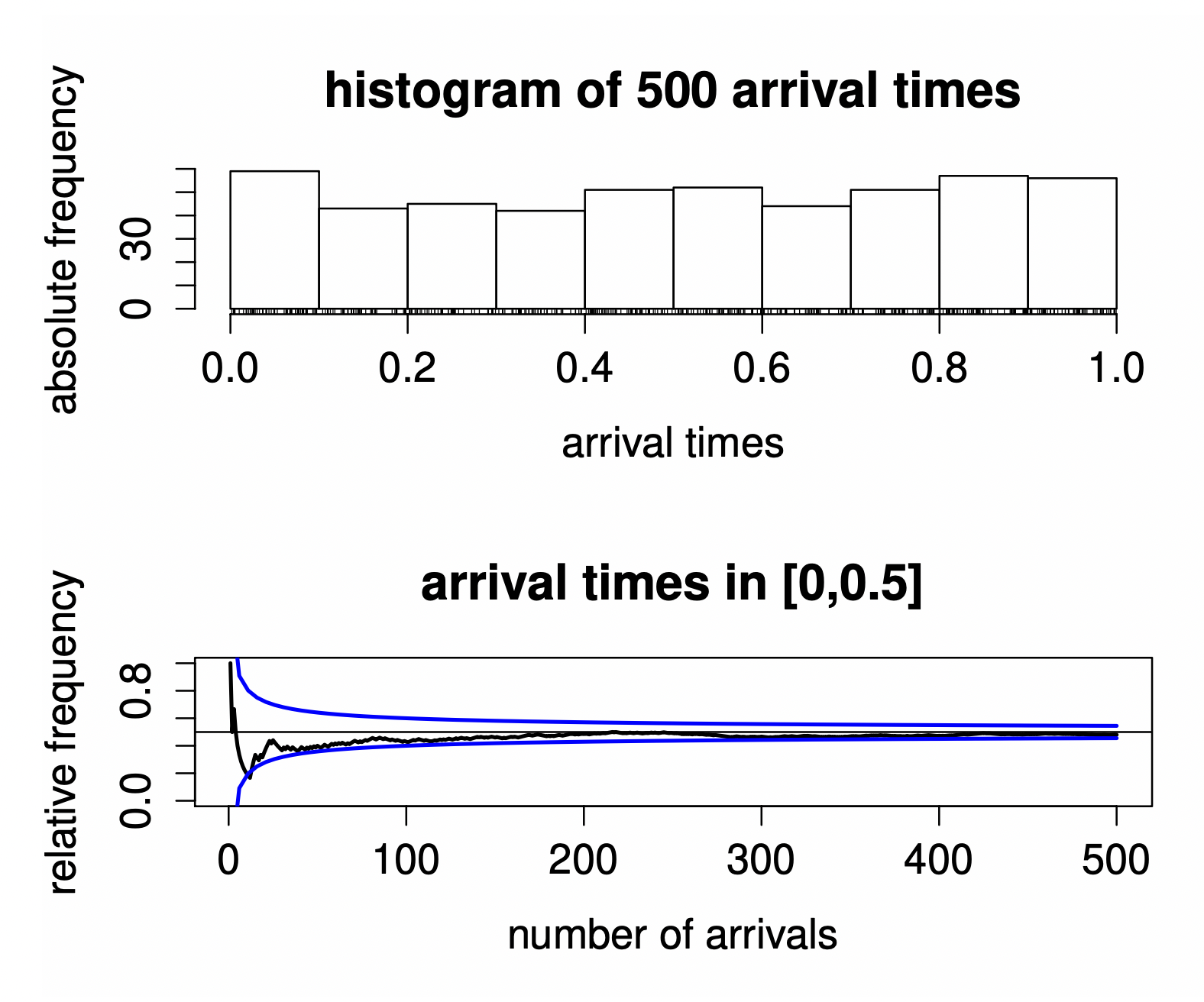
• Definition of Relative Frequency for Intervals
• Relative Frequencies always uniform convergent for every interval
• We use the limit of Relative Frequency to define the probability.
• Estimate Error → Unknown probability mostly (has to be quantified by percentage) in Confidence Interval $\left[h_n(I)-1/\sqrt{n},h_n(I)+1/\sqrt{n}\right]$

We can use a Barplot or Histogram to plot frequencies of items. We can describe the probability for every interval in an ECDF.

Relative Frequency convergence

• Coint Tossing where relative and interval frequencies always converge to $\frac{1}{2}$
• Arrival times in $[0,1]$

CDF to PDF relation.

→ Infer it from the data (Calculate every p-quantile)

Chapter 3 - Random Variables

For real random Random Variables we mostly have events as intervals or sets (in this case they are generated by repeated application of unions and complementations of intervals). The set of all these intervals is called the Borel Sigma Algebra of $\mathbb{R}$ on which we can define the Probability Measure which goes to $[0,1]$ from an event out of the Borel Sigma Algebra.

$$F_Y(t):=\mathbb{P}(Y\le t)=\mathbb{P}\left(Y^{-1}((-\infty ,t])\right)$$

Identity Map The probability of the identity map for $t$ is $F(t)$.

Linear Transformation $F_Z(t)=P(a+bY\le t)=P(Y\le (t-a)/b)=F_Y((t-a)/b)$ where $Z=a+bY$ ECDF: Let there be a data sequence with Item Expression (ordered values) ${\zeta }_1<...<{\zeta }_k$ and frequencies $n_1,...,n_K$.

$P(Y\le t)={\sum }_{j:{\zeta }_j\le t}P(Y={\zeta }_j)=F_n(t;x)$

p-Value Statistical Simulation

Chapter 5 - Estimators

We would like to extend CDFs to vector valued items. That way we can for example repeat the same experiment multiple times.

So we describe such a repeated experiment with a Random Variable $X$ where every $X_i$ is a specific observation of that experiment.

We can define the CDF like this:

$F\left(t_1,\dots ,t_n\right)=\mathbb{P}\left(X\in \left(-\infty ,t_1\right]\times \dots \times \left(-\infty ,t_n\right]\right)=\mathbb{P}\left(X_1\le t_1,\dots ,X_n\le t_n\right)$

If all random variables are independent we can write: $\mathbb{P}\left(X_1\le t_1,\dots ,X_n\le t_n\right)=F\left(t_1\right)\cdot \dots \cdot F\left(t_n\right)$ This also implies $\mathbb{E}\left(X_i{X}_j\right)=\mathbb{E}\left(X_i\right)\mathbb{E}\left(X_j\right)\text{ for }i\ne j$ which implies uncorrelatedness.

We can use Standard Estimators to estimate Expectation, Variance and CDF from a data sample.

Chapter 6 - Gauß Test

General

Null Hypothesis and Alternative

• Type 1 Error
• Type 2 Error
• Requirement: Type 1 and 2 Error probability $\alpha \in (0,1)$ should be small.

However typically $n$ isnt large enough which is why you often have to give up the requirement of a low Type 2 Error.

We can use a Power Function to describe a tests error rates and power.

• Test Statistic
• Gauß Test
• Planning Test Size

Robustness

Test Statistic (standardized mean or other metrics/estimators) needs to be normally distributed. → Zentraler Grenzwertsatz.

For any arbitrary CDF with Expectation $\mu$ and Variance ${\sigma }^2$ we can apply the Central Limit Theorem. Thus the estimated mean is normally distributed and we can estimate ${\sigma }^2$ from a sample.

→ Apply Gauß Test

This strategy also works for other Standard Estimators and similar tests can be developed.

General Confidence Intervals for Gauß Tests

We have with probability $1-\alpha$:

$$\begin{array}{c}\mu \in \left(-\infty ,{\bar{X}}_{(n)}+z_{1-\alpha }\frac{\sigma }{\sqrt{n}}\right],\mu \in \left[{\bar{X}}_{(n)}-z_{1-\alpha }\frac{\sigma }{\sqrt{n}},\infty \right)\\ \mu \in \left[{\bar{X}}_{(n)}-z_{1-\alpha /2}\frac{\sigma }{\sqrt{n}},{\bar{X}}_{(n)}+z_{1-\alpha /2}\frac{\sigma }{\sqrt{n}}\right]\end{array}$$

Chapter 11 - Distribution Parameters cont’d

Plug-In-Method Maximum Likelihood Estimation

Chapter 12 - Curve Fitting

• We have a data sequence and want to find a function that best describes it.
• “Best describing” can be quantified using an error metric.

Relative Error

Relative Error

Relative Error

Normalized and thus comparable for different $n$. $E_f(x,t):=\frac{1}{n}\Vert x-f(t)\Vert$

Measures the vertical distance between data points. If both $x$ and $t$ contain errors, use Euclidean Distance instead.

For Time Series Data a Dynamic Time Warping algorithm might be important.

Link zum Original

We now want to find or choose a function that minimizes this error. This method is also known as the Method of Least Deviation. This method doesn’t necessarily result in a unique minimal error (if at all minimal error) as often only numerical solutions exist.

This method leads to Least Squares Method which is a popular way of solving the described problem.

$\hat{f}$ is also called the regression function.

The Residuum can be used to study the underling random mechanisms.

Definition of the problem We can choose a function $f$ from a set of all possible polynomials.

• Linear Model
• Exponential Growth
• Allometric Growth

Least Squares This method uses a Linear Model and the least squares error function.

$\Vert x-A(t)\cdot \gamma {\Vert }_2$ See Mean Squared Error for more details.

Solutions depend on the complexity of the model which is mostly determined by the dimensions of $\gamma$ :

• Arithmetic Mean for $s=1$
• Simple Linear Regression for $s=2$
• Polynomial Regression for $s=d+1$
• Multiple Linear Regressions for $s=d+1$

Linear Gaussian Model

Geometric View

From the geometric view, the least squares method can be understood as an orthogonal projection

Illustration

Simple Linear Regression

The method is often numerically stable, even for non-linear models.

Chapter 17 - Limit Theorems and Simulations

In this first subchapter we learn about the Strong Law of Large Numbers which we can use to define the Glivenko-Cantelli theorem.

The fundamental theorems become important when we want to talk about Kolmogorov in the next subchapter.

In this subchapter we define a general goodness of fit test that can test wether the unknown Distribution of a data sequence euqals some distribution $G$.

We can use this general approach to definde the Kolmogorov Smirnov Test which uses the Kolmogorov Distribution for its Test Statistic.

Furthermore we can use the Lilliefors Test of Normality to determine whether a data sequence from an unknown distribution falls into the class of normal distributions,