Log-Likelihood
Because small values are very unstable in computers, we use the Log-Likelihood. It uses a sum and applies the logarithm to every datapoint.
L(θ)=i=1∏Np(si∣θ)=∗i=1∑Nlog[p(si∣θ)]=ℓ(θ)
Rewrite Log-Likelihood by inserting the Logistic Function and applying the logarithm to the sum
L(θ)=log(i=1∏mP(yi∣xi))=i=1∑mlog(g(θ⊤xi)yi(1−g(θ⊤xi))1−xi)
then again applying the logarithm to the exponents
=i=1∑myilog(g(θ⊤xi))+(1−yi)log(1−g(θ⊤xi))
then using the definition of the Logistic Function to get
=i=1∑myilog(1+eθ⊤xieθ⊤xi)+(1−yi)log(1+eθ⊤xi1)=i=1∑myiθ⊤xi+log1+eθ⊤xi1
and finally using the definition again to get
=i=1∑myiθ⊤xi+log(1−g(θ⊤xi))
We can use this much simpler form of the equation to calculate the Gradient of the Log-Likelihood:
∇θL(θ)=∇θ(i=1∑myiθ⊤xi+log(1−g(θ⊤xi)))=i=1∑myixij+1−g(θ⊤xi)1(−g(θ⊤xi)(1−g(θ⊤xi))xij=i=1∑myixij−g(θ⊤xi)xij=i=1∑m(yi−g(θ⊤xi)xij
and the Hessian Matrix like this
∇θ∇θL(θ)=∇θi=1∑m(yi−g(θ⊤xi)xij=i=1∑m−g(θ⊤xi)(1−g(θ⊤xi))xixi⊤
We can now use the Newton Method to iteratively calculate the best parameters:
θk+1=θk−(∂θ∂θT∂2L(θk))−1∂θ∂L(θk)
For Gaussian
We then insert the Gaussian Distribution of y like this:
i=1∑Nlog[p(si∣θ)]=i=1∑Nlog[(2πσ21)21e−2σ21(yi−wTxi)2]=−2σ21i=1∑N(yi−wTxi)2−2Nlog(2πσ2)
The Log-Likelihood can then be simplified to a negative constant times the ==Residual Sum of Squares (Also called the Loss)== and adding another constant at the back.
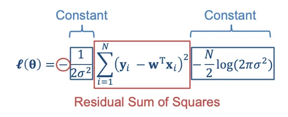
We now have a minus sign in the front. That is why we have to minimize the Residual Sum of Squares to maximize the Log-Likelihood.
The Loss is convex thus it has a unique minimum which can be calculated with: