Partial Dependence Plot

Definition

The marginal effect one or two features have on the predicted outcome of a ML model.

A partial dependence plot can show whether the relationship between the target and a feature is linear, monotonic or more complex. For example, when applied to a linear regression model, partial dependence plots always show a linear relationship.

$S$ is a subset of features (one or two) that are independent with the others. $C$ are all other features that are not in $S$ . We assume that all features in $C$ are uncorrelated with the ones in $S$ .

The partial dependence is

\hat{f}_S\left(x_S\right)=E_{X_C}\left[\hat{f}\left(x_S, X_C\right)\right]=\int \hat{f}\left(x_S, X_C\right) d \mathbb{P}\left(X_C\right).

We can estimate this integral using the Monte-Carlo for Integrals method. We then get the simple average over all data points where we fix the values in $S$ to the value from $x$ .

\hat{f}_S\left(x_S\right)=\frac{1}{n} \sum_{i=1}^n \hat{f}\left(x_S, x_C^{(i)}\right).

PDP-based Feature Importance

We can use the flatness of the PDP to determine the Feature Importance.

flat → low importance
high Variance → high importance

I\left(x_S\right)=\sqrt{\frac{1}{K-1} \sum_{k=1}^K\left(\hat{f}_S\left(x_S^{(k)}\right)-\frac{1}{K} \sum_{k=1}^K \hat{f}_S\left(x_S^{(k)}\right)\right)^2}

Examples

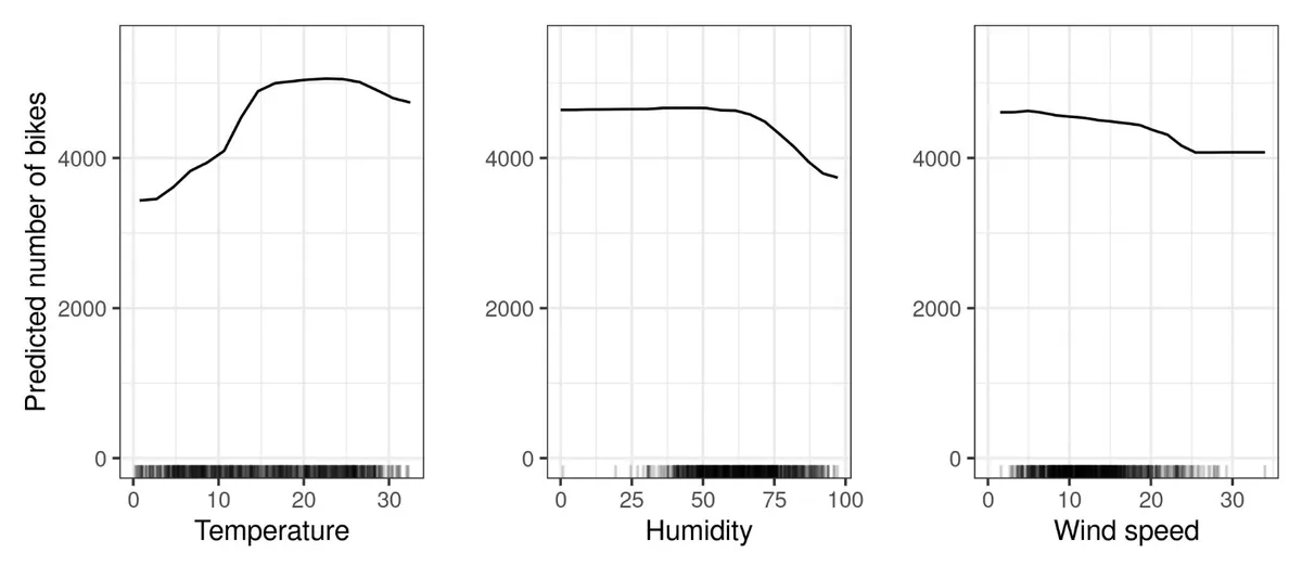
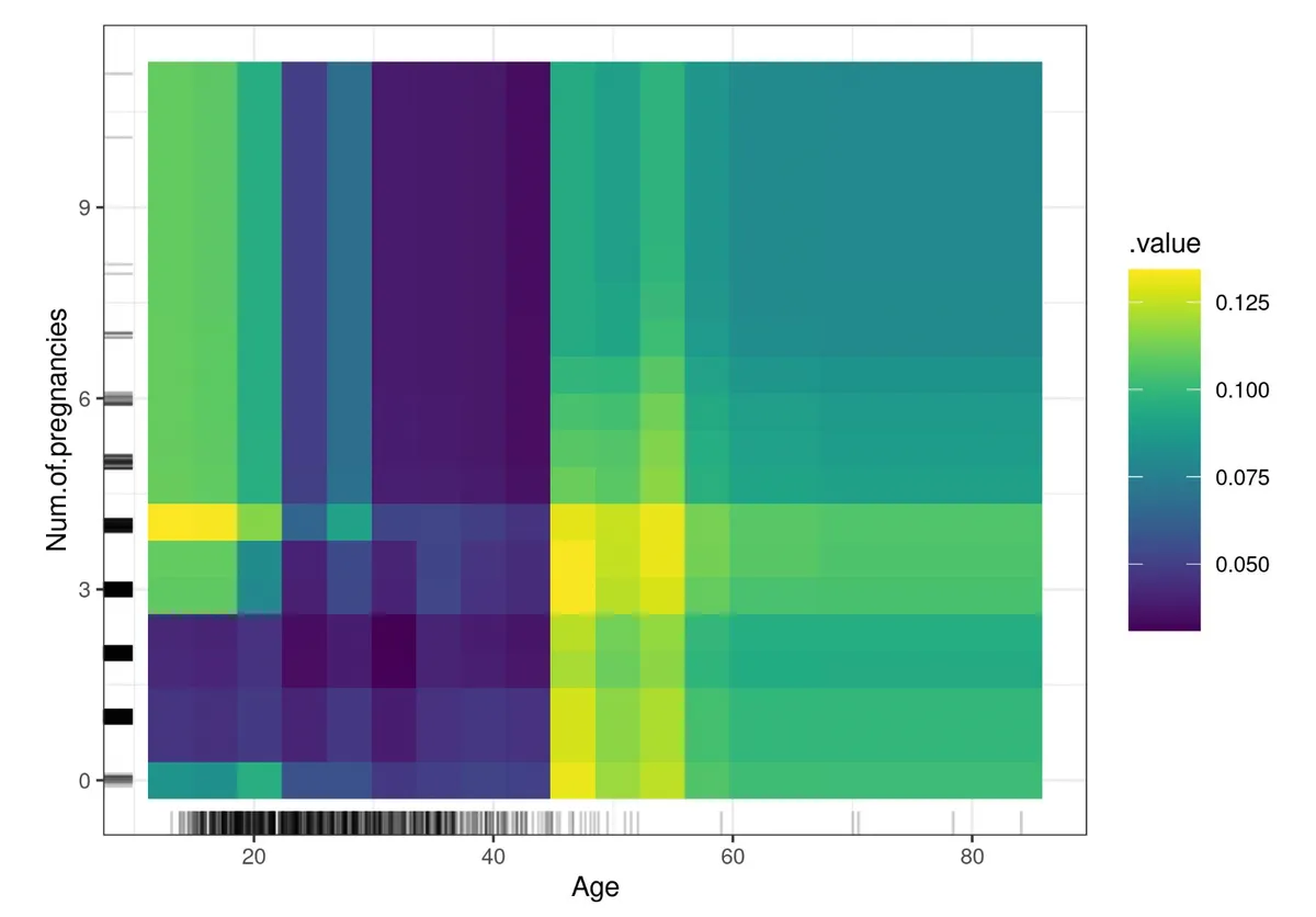
Bildschirmfoto 2023-07-03 um 12.28.26.png

For more than one feature you can use a Heatmap: Bildschirmfoto 2023-07-03 um 12.28.43.png

Pros

intuitive
clear interpretation
easy to implement
"causal" interpretation (at least in the model context, not in the real world though)

Cons

maximum of two features
assumption of independence with other features
- else there might be data points that are extremely unlikely (see rug plot)
- → use Accumulated Local Effect Plot
heterogeneous effects might be hidden
- → use Individual Conditional Expectation Curve
dont show feature distribution
- → use rug plot (see example)

In sklearn

Implemented + you can use PDPBox