Friedman's H-statistic

If there is no interaction we can decompose the PDP into

P D_{j k}\left(x_j, x_k\right)=P D_j\left(x_j\right)+P D_k\left(x_k\right)

and the prediction function into

\hat{f}(x)=P D_j\left(x_j\right)+P D_{-j}\left(x_{-j}\right).

Here $-j$ means all features that are not $j$ .

The two statistics are

H_{j k}^2=\frac{\sum_{i=1}^n\left[P D_{j k}\left(x_j^{(i)}, x_k^{(i)}\right)-P D_j\left(x_j^{(i)}\right)-P D_k\left(x_k^{(i)}\right)\right]^2}{\sum_{i=1}^n P D_{j k}^2\left(x_j^{(i)}, x_k^{(i)}\right)}

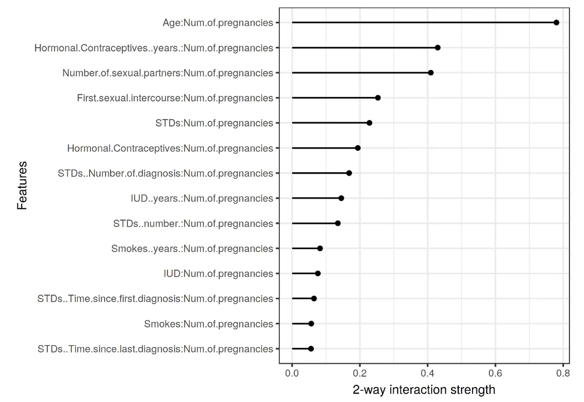
(interaction of feature $j$ with $k$ ) and

H_j^2=\frac{\sum_{i=1}^n\left[\hat{f}\left(x^{(i)}\right)-P D_j\left(x_j^{(i)}\right)-P D_{-j}\left(x_{-j}^{(i)}\right)\right]^2}{\sum_{i=1}^n \hat{f}^2\left(x^{(i)}\right)}

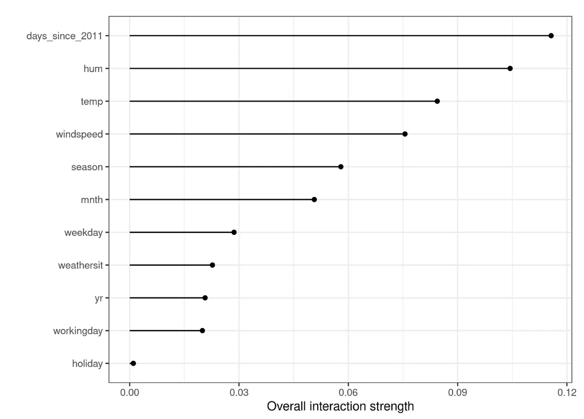
(interaction of feature $j$ with all other features).

The statistic is expensive to evaluate, it takes $2n^2$ and $3n^2$ calls to the model.

Examples

Bildschirmfoto 2023-07-11 um 11.28.41.png

Pros

Cons